Markowitz Efficient Frontier - An introduction with Python

According to Investopedia, Efficient Frontier is:

The efficient frontier is the set of optimal portfolios that offers the highest expected return for a defined level of risk or the lowest risk for a given level of expected return. Portfolios that lie below the efficient frontier are sub-optimal, because they do not provide enough return for the level of risk. Portfolios that cluster to the right of the efficient frontier are also sub-optimal, because they have a higher level of risk for the defined rate of return.

Investopedia

It’s described on Harry Markowitz paper from 1952.

Let’s learn how to apply Python library to study the Efficient Frontier of two assets.

First, we’ll need to import the libraries:

import numpy as np
import pandas as pd
from pandas_datareader import data as wb
import matplotlib.pyplot as plt
%matplotlib inline

Let’s grab some data from the B3, Brazilian stock exchange. For that, we’ll need the code of the exchange (BVMF) and the tickers of the stocks. For this example we’ll study AmBev (BVMF:ABEV3) and Itaú (BVMF:ITUB3).

Pandas has a feature called DataReader that can get financial data from some sources, including Google Finance.

assets = ["BVMF:ABEV3", "BVMF:ITUB3"]
bvmf_data = pd.DataFrame()
for t in assets:
    bvmf_data[t] = wb.DataReader(t, data_source='google', start='2009-1-1')['Close']

We need to normalize the returns of the stocks. They have different prices, but what is important on this study, are their returns (the variation of the prices). Let’s use the log function from numpy to achieve this.

log_returns = np.log(bvmf_data / bvmf_data.shift(1)) # Normalizing returns by using log

Besides choosing stocks when managing a portfolio, we have to decide the asset allocation. Let’s create a function that produces a random allocations (in %). This will be used later on our study.

def rand_weights(n):
    '' Produces n random weights that sum to 1 ''
    weights = np.random.rand(n)
    weights /= np.sum(weights)
    return weights'

Here is our study. Let’s create 10.000 random portfolios, get their annual returns (250 days) and their volatilities. Then we’ll create a DataFrame with the results to plot that data.

pfolio_returns = []
pfolio_volatilities = []

for x in range (10000):
    weights = rand_weights(len(assets))
    pfolio_returns.append(np.sum(weights * log_returns.mean()) * 250)
    pfolio_volatilities.append(np.sqrt(np.dot(weights.T,np.dot(log_returns.cov() * 250, weights))))

pfolio_returns = np.array(pfolio_returns)
pfolio_volatilities = np.array(pfolio_volatilities)

portfolios = pd.DataFrame({'Return': pfolio_returns, 'Volatility': pfolio_volatilities})

And here is the Markowitz Efficient Frontier:

portfolios.plot(x='Volatility', y='Return', kind='scatter', figsize=(10, 6));
plt.xlabel('Expected Volatility')
plt.ylabel('Expected Return')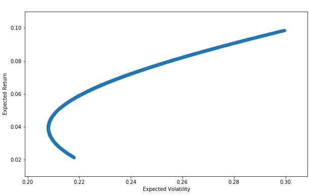

The full notebook can be seen at my Github.